A graphical exploration of power, type S, and type M errors

Tl;dr

I discuss:

What are "type M" and "type S" errors
How they have a simple graphical interpretation
How these errors change if the effect size itself is uncertain: a form of "prior sensitivity"

Introduction

In traditional statistical testing, we often report p-values. These represent the probability of making a “type I” error: incorrectly concluding there is a difference between treatment and control (rejecting the “null hypothesis”), when there actually isn’t. Yet, as many have argued, “type II” errors — failing to conclude there is an effect, when there actually is — can be just as important. Type II errors are related to “statistical power”: the probability of detecting a real effect, if it exists.

There are (at least) three reasons we should care about statistical power:

With low power, we are unlikely to find a statistically significant result
1. We don’t want to waste time running an experiment, which is typically a large investment of resources, if it cannot detect the kinds of effects we’re interested in
And, even if we do find a statistically significant result:
1. Its magnitude is likely exaggerated (”magnitude exaggeration”)
2. For severely underpowered test, the observed effect might even be of the wrong sign (”sign error”)

What I termed “magnitude exaggeration” is better known as the “winner’s curse”. As Ron Kohavi explains:

When the power is low, the probability of detecting a true effect is small, but another consequence of low power, which is often unrecognized, is that a statistically significant finding with low power is likely to highly exaggerate the size of the effect. The winner’s curse says that the “lucky” experimenter who finds an effect in a low power setting, or through repeated tests, is cursed by finding an inflated effect.

Andrew Gelman and John Carlin introduced a useful framework for think about the consequences of underpowering in their 2014 paper “Beyond Power Calculations: Assessing Type S (Sign) and Type M (Magnitude) Errors”. They refer to “magnitude exaggeration” as a “type M” error, and the “sign error” as a “type S” error.

These quantities are especially useful in “retrospective analysis”: when we analyze, after the fact, the statistically significant result from an A/B test. The type S error tells us if we’re making the correct decision by believing that the winning variant was indeed better. The type M error tells us by how much we’re inflating the magnitude of the reported win. For example, suppose the power is 50%. The corresponding type M error is 1.41, so an observed effect of, say, 10% should likely be adjusted down to 7.1% (=10%/1.41) or so.

Doing retrospective analysis is often useful, but type M and type S errors can be difficult to explain to others. Below is my attempt to illustrate the intuition behind these errors. I also talk about how we might extend this analysis when the true effect sizes are uncertain (which is usually the case).

Code

As usual, I’m going to simulate my way to the solution instead of relying on derivations. (This is also the approach Gelman and Carlin adopt in their paper; see their retrodesign function.) The code is in this Google Colab notebook, and most of the functions are simply copied from this previous blog post of mine.

Here’s the basic idea:

Assume a particular "true" effect size. (The magnitude is unimportant; only the ratio of the effect size to the standard error matters.)
Do a standard power calculation to get the sample size required to power the A/B test to a prescribed power (say, 80%).
Run a set of simulations (Monte Carlo trials) to generate treatment and control samples, according to the effect size (here, samples are drawn from normal distributions, but this isn’t essential)
From each trial, produce the following quantities:
1. The observed effect size: the difference between the mean of the treatment and control samples
2. The standard error of the effect size
3. The p value
4. Whether the result is statistically significant (here, p < 0.05, two-sided)
Confirm, using Gelman and Carlin’s retrodesign function, whether the retrospectively computed power agrees with the prescribed power.

Here’s my re-implementation of retrodesign, for example (note: I’m operating under the large N case where we can use the Gaussian distribution instead of Student t):

import numpy as np
from scipy.stats import norm

rng = np.random.default_rng()

def retrodesign(pre_experiment_effect_size, standard_error, alpha=0.05, n_sims=10000):
    normalized_effect = pre_experiment_effect_size / standard_error
    z_crit = norm.ppf(q=1 - alpha / 2)
    p_hi = 1 - norm.cdf(x=z_crit - normalized_effect)
    p_lo = norm.cdf(x=-z_crit - normalized_effect)
    power = p_hi + p_lo
    typeS = p_lo / power
    normalized_estimate = normalized_effect + rng.normal(loc=0, scale=1, size=n_sims)
    significant = np.abs(normalized_estimate) > z_crit
    exaggeration = max(
        1.0, np.mean(np.abs(normalized_estimate)[significant]) / normalized_effect
    )

    return {
        "magnitude_error": exaggeration,
        "power": power,
        "sign_error": typeS,
    }

From the results of the simulations, it’s also easy to calculate the type M and type S errors. Here’s that snippet:

frame = (
    frame
    # these errors are computed for only statistically significant results
    .query("stat_sig")
    .assign(
        exaggeration=lambda x: x["observed_effect_size"] / x["true_effect_size"],
        sign_error=lambda x: np.sign(x["observed_effect_size"])
        != np.sign(x["true_effect_size"]),
    )
    # group by a relevant variable (here, the power)
    .groupby(by=["power"])
    # type M errors are usually computed using the mean,
    # but the median can also be informative
    .agg(
        type_m_mean=pd.NamedAgg("exaggeration", "mean"),
        type_m_median=pd.NamedAgg("exaggeration", "median"),
        type_s=pd.NamedAgg("sign_error", "mean"),
    )
)

Graphical exploration

Let’s explore a range of values for the prescribed power: 80%, 50%, 20%, and 10%

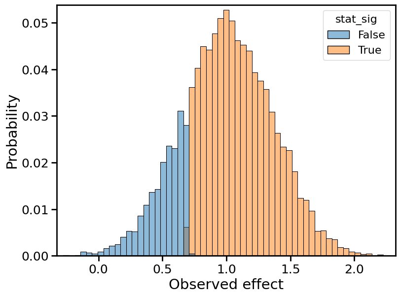
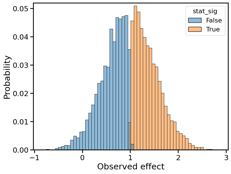
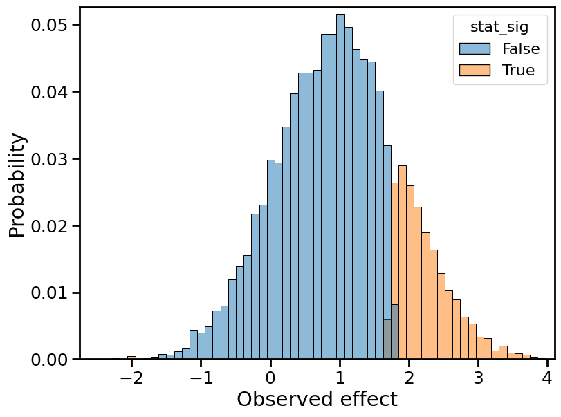
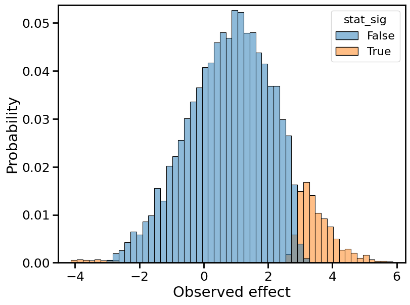
Below, I plot histograms of the observed effect size, normalized by the true effect size, for 10,000 Monte Carlo trials. Each plot depicts two histograms: one for the statistically significant results (in orange), the other for the non statistically significant results (in blue).

Observed effects for 80% power

Observed effects for 50% power

Observed effects for 20% power

Observed effects for 10% power

What happens as the power decreases?

The overall distribution, combining orange and blue, remains centered on the true effect size (1, in normalized terms). This is because the observed effect is still an unbiased estimator of the true effect. Moreover, the shape of the overall distribution remains roughly Gaussian, which is a consequence of the central limit theorem.

While certain aspects of the distribution remain the same, one important statistic does not: the width. The distribution becomes wider, and its variance increases. In statistical terms, we’d say the “standard error” of the observed effect is increasing. (Again, a consequence of the central limit theorem/law of large numbers.)

At the same time, the ratio of orange (stat-sig) to blue (non stat-sig) decreases. In fact, the proportion of orange mass is simply the power. At 50% power, we should observe a statistically significant effect half the time, so the “mass” of the blue distribution must equal the mass of the orange distribution.

The type M error is the mean of the orange distribution. To avoid type M errors (”exaggeration”), we’d like the orange distribution to lie as close to 1 as possible. Using that fact, let’s try to explain the “winner’s curse” or, equivalently, why type M errors increase with decreasing power.

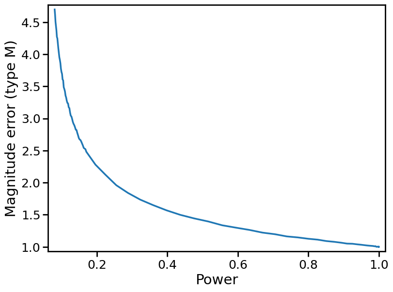
In fact, either of the effects described above — increasing standard error, or shifting proportion of “orange” to “blue” — would result in the winner’s curse. If the standard error increases, the orange effects we are measuring are pushed outwards, further away from the true effect size. And if the proportion of orange mass decreases, then the statistically significant effects we are measuring are necessarily larger in magnitude. But, combined together, both phenomena imply a rapid increase in the type M error as power decreases. In fact, this is what we see in Figure 2 of Gelman and Carlin’s paper (reproduced below).

Type M error vs. power

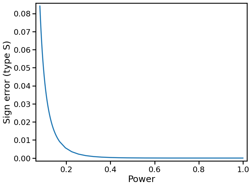
Similar explanations hold for the type S error. The distribution gets pushed outward, which means that the left tail approaches increasingly negative values. The type S error is the proportion of the orange distribution that lies below 0. It is negligible when power ≥ 50%, but starts to crop up in the 20% power plot, and even more so in the 10% power plot.

Type S error vs. power

When the true effect size is uncertain

So far we’ve discussed the case where the true effect size is certain. The alternative hypothesis is a “spike” (at effect = true effect size), just like the null hypothesis is a spike at effect = 0. Gelman and Carlin also talk about the more typical case where the true effect size is uncertain. They write:

Like power analysis, the design calculations we recommend require external estimates of effect sizes or population differences. Ranges of plausible effect sizes can be determined on the basis of the phenomenon being studied and the measurements being used. One concern here is that such estimates may not exist when one is conducting basic research on a novel effect. When it is difficult to find any direct literature, a broader range of potential effect sizes can be considered.

How would the type M/type S analysis change if we had a range or distribution of true effect sizes, instead of a solitary spike? For simplicity, we can take a uniform distribution with some width, centered on the true effect size we used earlier. Again, this is fairly easy to simulate: instead of taking the true effect as fixed, we draw it from some “prior” distribution: here, a uniform one.

It turns out that, in this case, the type M error decreases, while the type S error increases. The scatterplot below reveals why (for a nominal prescribed power = 50%). It is the observed effect size vs the true effect size (again, for 10,000 Monte Carlo simulations).

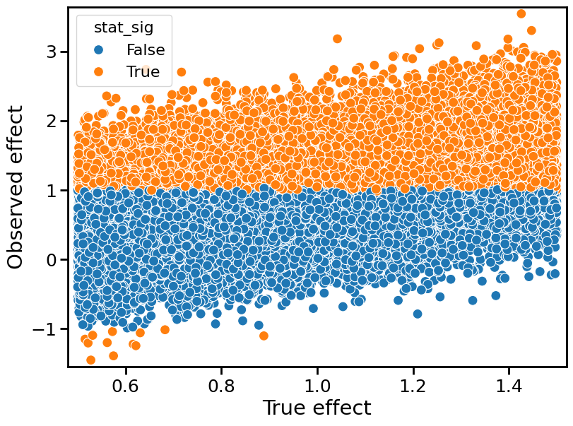
50% power, uncertain true effect size

The type M error, for a range of true effect sizes, is a weighted average of the individual type M errors at a given effect size. The weights are proportional to the prior distribution (here, uniform) and the probability of observing a statistically significant result (the power). When we consider a range of true effect sizes, the larger effect sizes correspond to higher values of power, so they count for more in the weighted average. Therefore, the type M error ends up being “skewed” towards larger effect sizes as well. Because the type M error decreases as the true effect size increases, the overall (weighted-average) type M error goes down as the true effect size becomes more uncertain.

Put more concisely: if you observe a statistically significant result, it is more likely to arise from a larger true effect, for which you should be overpowered (have more power than the nominal prescribed power).

Conversely, the type S error increases as the uncertainty in true effect size increases. Again, the plot above reveals why. The type S error (orange dots lying below 0 on the y-axis) only crops up for small true effect sizes, at the left of the prior distribution. In this case, we are underpowered. If we know, a priori, that small true effect sizes are impossible, then we will never be underpowered, and the type S error will be 0. But this only happens when the true effect size distribution is close to a spike. In other, more realistic cases, the true effect is uncertain, and type S errors will be non-negligible.

This finding is related to the fact (discussed in another blog post of mine) that the probability of a false positive can be large if the prior probability of the null hypothesis is large.

In both cases, a large proportion of the “mass” of the prior effect distribution lies close to 0. So, we might incorrectly conclude a positive result when a null or negative result is actually the case, or vice versa. Effectively, these are “probabilities of making a false positive error” (also known as false positive risk) and “type S” errors, respectively.

Both the type S/type M framework and Kohavi's "false positive risk" analysis depend on priors for the effect size distribution. In the former case, the prior is the range of plausible effect sizes. In the latter case, it's the probability that the null hypothesisis is true. One key takeaway is that “prior sensitivity” is important in either case (and, in fact, these frameworks are closely related). Quantities like false positive risks and type M/type S errors can be quite sensitive to the magnitude and spread of the prior effect size distribution.

Conclusion

Type S and type M errors are a useful framework for thinking about statistically significant results from A/B tests. They allow us to assess whether these results are inflated in magnitude (”winner’s curse”) and/or incorrect in sign. In graphical terms, these errors are fairly easy to express. The statistical power is the proportion of overall “mass” in the “orange” (statistically significant) distribution. The type M error is the average value within the orange distribution. And the type S error is the proportion of mass in the orange distribution lying below 0. By exploring how these distributions change as the power changes, we gain deeper intuition about these errors. In particular, we learned that there are two effects driving these errors higher as power diminishes: first, the increase in standard error (for a fixed effect size), and second, the shifting mass between “orange” (stat sig) and “blue” (non-stat sig) distributions. When combined, they cause the type M and type S errors to rise nonlinearly with decreasing power.

We also looked at what happens when the true effect size is uncertain: not a “spiky” alternate hypothesis, but instead a range of effect sizes. Here the results are somewhat more complicated, but the intuition from the scatterplot of observed vs. true effect sizes is helpful. We found that, as small true effect sizes become likelier, it becomes correspondingly difficult to avoid making a type S (sign) error. In general, type S/type M errors are susceptible to the same kind of “prior sensitivity” that affects other quantities reported in A/B testing, like the false positive risk.

Statistical power should be thought of in reference to a true effect size. The same sample that guarantees 80% power with an effect size of 1 will likely not guarantee adequate power with an effect size of 0.1. Unfortunately, this means that if the true effect size is highly uncertain, or we know it lies close to 0, we cannot simply "assume away" type M/type S errors.