A random walk down Wall Street
Introduction
I was lucky enough to receive an offer from a tech company recently, and, as part of that offer, a substantial equity package. This company allows you to choose your own mix of equity. The equity package can be allocated across four asset types: cash, restricted stock units (RSUs), and two types of options, one aggressive ("at the money", or ATM) and the other very aggressive ("out of the money", OTM). The value of the equity package, for the non-cash asset types, depends on how the stock price evolves during one's tenure. If the stock price increases greatly, the OTM and ATM options are superior to RSUs, which in turn is superior to cash. If the stock price drops, the ranking is reversed. While the HR department provided a helpful guide to understand the mechanics of each asset type, and informed me that, if I couldn't make a decision, I would be opted-in to a mix of 75% RSUs and 25% ATM options, I wanted to understand the value of this package in greater detail. (The term "value" is ill-defined, and I'll return to it later.)
I decided to tackle this problem using simulation. The system being modeled can be divided into a few pieces: the actor (me), the equity package, and the stock price. Some of these, like the stock price, evolve endogenously, according to their own mechanics. (Presumably, I am a small enough actor that, while the stock price affects my decisions, like whether/when to exercise, my decisions do not affect the stock price.) Typically, these mechanics will be parametrized by random variables. For instance, as I'll discuss below, we can assume the stock price changes according to a "geometric Brownian motion" process in which there is a long-term, deterministic trend (parametrized by $\mu$) and short-term, stochastic volatility (parametrized by $\sigma$). I do not know the true values of $\mu$ or $\sigma$, and, if I did, I would be a retired multimillionaire instead of a humble blogpost writer. Instead, I have a rough idea of what reasonable values these parameters might take, based both on historical data as well as my knowledge of trends in the broader market.
Running the simulation involves stepping from time $t$ to time $t+1$, and repeating this process $N$ times. What happens during each step? The stock price changes according to the mathematical model. Some of my equity vests. If that equity represents RSUs, I have a decision of whether or not to sell it immediately, or to hold it. And, if that equity represents options, I can choose to exercise and sell immediately, exercise and hold, or not exercise at all. The range of possibilities is actually quite daunting, and expands geometrically with each time increment. In what follows, I will make some (grossly) simplifying assumptions, but, in general, if we want to determine the actor's optimal decision over a range of simulations/scenarios, we need to optimize over the entire space of his/her decisions. In this example, that means optimizing both for the initial allocation decision --- what fraction of cash, RSUs, and options to choose --- and for the decision about exercising and selling at each time step.
How does the "optimization" actually happen? This is actually quite complicated! One plausible approach, although by no means the only one, is to take the results of each simulation and assign a "utility" to each. I would have a function, $U(M_i)$, that describes my utility, $U$, corresponding to the money, $M_i$, generated from simulation $i$. This curve should be monotonically increasing, but need not be linear. Presumably my utility from making \$100k is not 10 times as much as making \$10k; there are diminishing returns to money. Then, the decision would be made on the basis of the actor's actions that maximize this expected utility. (This field of study is known as "Decision Theory", if you'd like to read more.)
To try to summarize, the following is a generic approach to "Monte Carlo" simulation-based decision making.
- Model the system mathematically, which means formulating an equation that describes the evolution of the system from time $t$ to $t+1$.
- The model will possess parameters that govern the system dynamics. Try to formulate a (multivariate) prior distribution for these parameters.
- Create a set of possibilities for rulesets that the actor in the simulation will follow.
- Arbitrarily assign the actor a single ruleset based on the possibilities enumerated above.
- Randomly draw a sample from the prior distribution.
- Run the simulation with these sampled parameters and the chosen actor ruleset. The simulation will involve repeatedly stepping through time. Store the results and use our function $U$ to compute the associated utility of the "possible future" that we have simulated.
- Repeat steps 5-6 sufficient times that we have confidence in our estimate of the expected value of utility for the actor ruleset being considered. This is known as the "Monte Carlo" approach. Note that this step can be very expensive, depending on how long it takes for each simulation to run, and how many simulations are required to reach "convergence".
- Repeat steps 5-7 for all possible actor rulesets.
- Maximize the expected utility with respect to the ruleset. Presumably, this is the ruleset we want to follow in practice. Of course, this recommendation is only as good as the assumptions that underpin it: the simplifications made in the mathematical model, the correctness of the prior distribution, the comprehensiveness of the possibilities for rulesets, etc.
All of this is somewhat abstract, so let's use my actual example to make these concepts more concrete.
Case study
Mathematical model
As mentioned above, there are three pieces here: the actor (me), the equity package, and the stock price.
The dynamics of the equity package are fairly simple. Excluding some minor details like the "equity cliff", at each timestep, a fraction 1/N of the equity vests. For instance, if the equity package is \$24k, and, assuming a 4 year vesting schedule, each month \$500 will vest. How this vesting translates into real money (and, in turn how that real money translates into "utility") is more complicated, and will be discussed later.
The stock price is assumed to follow a "Geometric Brownian Motion" model. This essentially decomposes the rate of return into two parts, one deterministic ($\mu$) and one stochastic ($\sigma$). The former describes how the stock price would evolve in the absence of volatility (the "drift"), and the latter accounts for the volatility. Because one of these terms describes a stochastic process, different simulations with the same set of parameters ($\mu$, $\sigma$) will give different results. The governing equation is:
$$ S_t / S_{t-1} = \exp(\mu - \sigma^2/2 + \sigma N(0, 1)) $$
where $S_{t}$ is the stock price at time $t$, and $N(0, 1)$ is a unit normal distribution.
(Important note: I do not work in finance, and I am certainly not an expert in financial modeling. I chose this model because it seemed widely used and reasonably tractable, but the assumptions of constant variance and Gaussian processes are known to be dubious, and I'm including this caveat so that Nassim Taleb doesn't yell at me.)
Actor's rulesets
There are two main decisons the actor makes. At $t = 0$, the actor decides how to allocate his/her equity across the four asset types: cash, RSUs, ATM options, and OTM options. Then, at each $t > 0$, the actor decides what to do with the equity that has vested. Let's cover each in turn.
Cash is very simple. Equity of amount $M_t$ vests at $t$, and the actor receives a "payout" of $0.9M_t$ in their bank account. (Note: The 0.9 factor is apparently related to tax reasons for the company. I am also ignoring taxation for the individual, which is a very big oversight, and, as a consequence, the numerical results below should not be taken as accurate. That being said, given the actor rulesets under consideration, the taxation of cash and RSUs is similar, so this effect is mostly irrelevant if options are not part of the allocation.)
RSUs are also fairly simple. At each time $t$, the actor receives a number of shares equal to $M_t / S_0$: i.e, the nominal value of the equity is divided by the stock price at the grant date, not at the vesting date. So, the actual value of these shares is $M_t * S_{t} / S_{0}$: the shares are worth more than cash (ignoring the discounting factor of 0.9) if the stock appreciates, and the shares are worth less if the opposite is true. I will assume that the actor is conservative, and will sell the RSUs immediately after vesting.
(This is not as stupid as it sounds: because RSUs are taxed on vesting, there is no real tax benefit to delaying the sale, and one can hedge against the company's stock by investing the proceeds into an index fund. In other words, we can imagine two scenarios: one in which we sell the shares and reinvest the same amount in the company (which is equivalent to holding); the other where we sell the shares and reinvest them in a diversified financial product. If the actor was given separate money for this, he/she would invariably choose the second option. So why should it be different if the actor is given money in the form of RSUs?)
Options are somewhat more complicated. Here I will make the somewhat questionable assumption that options are exercised at the end of the time period under consideration, with the caveat that they are not exercised if they are worthless. For ATM options, options are worth something if $S_{t} > S_{0}$: the stock has to appreciate. For OTM options, options are worth something only if $S_{t} > 1.5S_{0}$: the stock has to appreciate by at least 50%. To justify this extra risk relative to RSUs, 4 times as many ATM options are given as RSUs for a given equity amount, and the corresponding ratio is 8 for OTM options. The payouts end up being $4 (M / S_0) \max(S_{t_{end}} - S_0, 0)$ for ATM, and $8 (M / S_0) \max(S_{t_{end}} - 1.5 S_0, 0)$ for OTM, where $M$ is the total amount of equity (so, $NM_t$, where $N$ is the number of time steps).
Other rulesets are possible for options. The disadvantage of the one under consideration is that the tax bill will be enormous if the options are worth a significant amount, since the gains are concentrated in a single year instead of being more spread out. We can also imagine immediate exercise (which probably doesn't make sense, especially for OTM options), and exercise as soon as the options are worth a certain amount. These are more complicated to model, however.
For the initial allocation decision, I will assume a few different possibilities, summarized in the table below:
| Allocation Type | Cash | RSUs | ATM Options | OTM Options |
|---|---|---|---|---|
| Cash only | 1 | 0 | 0 | 0 |
| RSUs only | 0 | 1 | 0 | 0 |
| ATM only | 0 | 0 | 1 | 0 |
| OTM only | 0 | 0 | 0 | 1 |
| Default | 0 | 0.75 | 0.25 | 0 |
| RSUs + Cash | 0.5 | 0.5 | 0 | 0 |
| RSUs + Options | 0 | 0.5 | 0.25 | 0.25 |
| Even | 0.25 | 0.25 | 0.25 | 0.25 |
Python code
The python code to run the simulation and model the payouts is presented below. The version I present is vectorized, which makes the computation faster but also perhaps less readable. Note that, in general, it's easier to program these simulations step-by-step (advancing from $t$ to $t+1$), but this may less computationally efficient.
import numpy as np

class SimulationRunnerVectorized:
    def __init__(self, mu, sigma, n_steps, allocation, price=1):
        """
        Initialize using parameters (mu, sigma), actor rulesets (allocation), and number of timesteps.
        The initial stock price can be set to 1 without loss of generality
        """
        self.mu = mu
        self.sigma = sigma
        self.n_steps = n_steps
        self.grant_price = price
        self.price = price
        self.allocation = {
            equity_type: np.ones(n_steps, ) * amount
            for equity_type, amount in allocation.items()
        }

    def compute_prices(self):
        """Compute stock prices for all timesteps"""
        drift = np.random.normal(size=(self.n_steps,))
        rate_of_return = np.exp(self.mu - 1/2*self.sigma**2 + sigma*drift)
        prices = self.price*np.cumprod(rate_of_return)
        return prices

    def run(self):
        """Run simulation: compute stock prices given initial allocation; compute final payouts"""
        prices = self.compute_prices()
        payouts = calculate_payout(
            current_price=prices,
            grant_price=self.grant_price,
            allocation=self.allocation
        )
        return payouts
Here is the code for calculating the payouts from the simulation results
from typing import Callable, Dict

import numpy as np

def calculate_payout(prices: np.array, grant_price: float, allocation: Dict[str, Callable]) -> float:
    """Calculate payout by aggregating over all equity types"""
    payout = 0
    payout_funcs = {
        "cash": payout_cash,
        "rsus": payout_rsus,
        "atm_options": payout_atm_options,
        "otm_options": payout_otm_options,
    }
    for equity_type, amount in allocation.items():
        payout += payout_funcs[equity_type](prices, grant_price, amount=amount)
    return payout

def payout_cash(prices: np.array, grant_price: float, amount: float, discount: float=0.1) -> float:
    return amount * (1 - discount)

def payout_rsus(prices: np.array, grant_price: float, amount: float):
    n_shares = (amount / grant_price)
    return n_shares * prices

def payout_atm_options(prices: np.array, grant_price: float, amount: float, immediate_exercise: bool=False) -> float:
    n_options = (amount / grant_price) * 4
    if immediate_exercise:
        # this possibility is not considered in the blog post, but is included for illustration
        return n_options * np.maximum(current_price - grant_price, 0)
    else:
        return n_options * np.maximum(current_price[-1] - grant_price, 0)

def payout_otm_options(prices: np.array, grant_price: float, amount: float, immediate_exercise=False) -> float:
    n_options = (amount / grant_price) * 8
    if immediate_exercise:
        # this possibility is not considered in the blog post, but is included for illustration
        return n_options * np.maximum(current_price - 1.5 * grant_price, 0)
    else:
        return n_options * np.maximum(current_price[-1] - 1.5 * grant_price, 0)
And, finally, here is the code to run the simulation loop (over all the different actor rulesets and parameter possibilities):
from typing import Dict

import numpy as np
import pandas as pd

ALLOCATION_RULESETS = {
    "cash_only": {
        "cash": 1,
    },
    # (many rulesets omitted)
    "even": {
        "cash": 0.25,
        "rsus": 0.25,
        "atm_options": 0.25,
        "otm_options": 0.25
    },
}

def get_allocation(allocation_ruleset: str, amount: float) -> Dict[str, float]:
    frac_allocation = ALLOCATION_RULESETS[allocation_ruleset]
    return {
        equity_type: frac * amount for equity_type, frac in frac_allocation.items()
    }

results = []
n_steps = 48  # 4 years * 12 months
N_simulations = 1000  # chosen arbitrarily
for allocation_ruleset in ALLOCATION_RULESETS.keys():
    print(strategy)
    # divide total equity amount by number of time steps
    allocation = get_allocation(allocation_ruleset, amount=1/n_steps)
    for mu in np.linspace(-0.1/12, 0.2/12, 21):
        for sigma in np.linspace(0, 0.5/12, 21):
            for simulation_num in range(N_simulations):
                payouts = SimulationRunnerVectorized(
                    mu=mu, sigma=sigma, n_steps=n_steps, allocation=allocation
                ).run()
                results.append({
                    "mu": mu,
                    "sigma": sigma,
                    "simulation_num": i,
                    "strategy": strategy,
                    "payout": payouts.sum()
                })
results = pd.DataFrame(results)
Note: there is some tricky logic here related to time. The time increments are monthly, which means that $\mu$ and $\sigma$ should also be treated as monthly rates of return and monthly drifts, respectively. With the parameter ranges chosen above, we cover a range of annual rates of return from roughly -10% to 20%. The values for $\sigma$ are also arbitrary, but the minimum value is 0 (in which case the simulation is deterministic), and the maximum value is on the order of $\mu$, which should make sense intuitively.
Simulation results
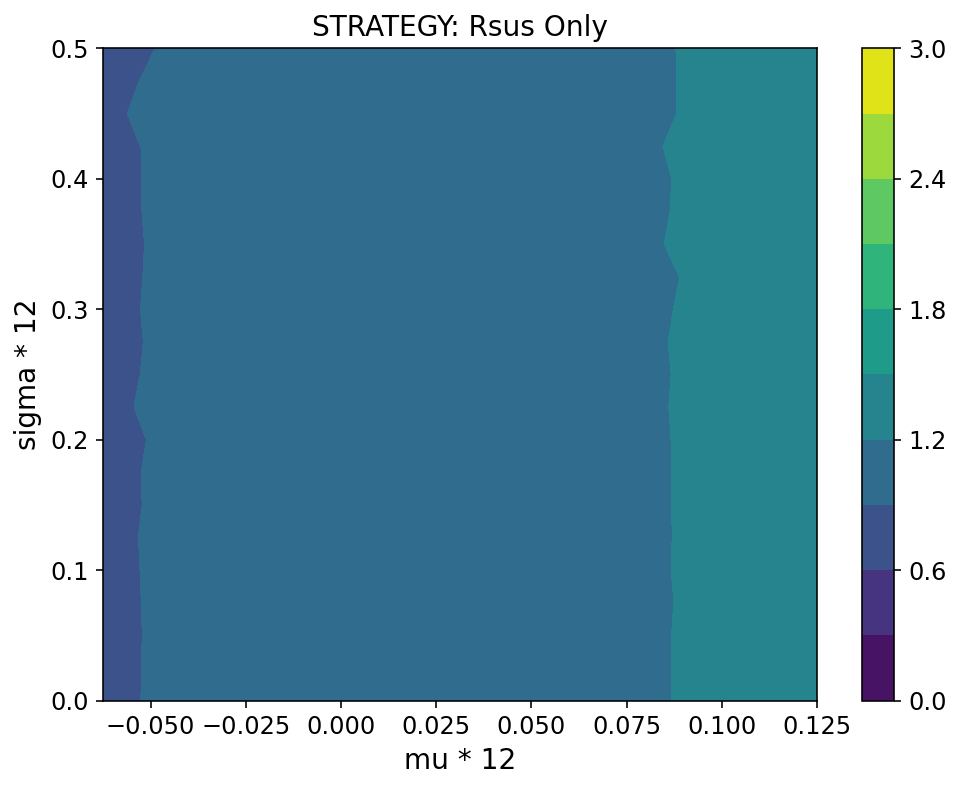
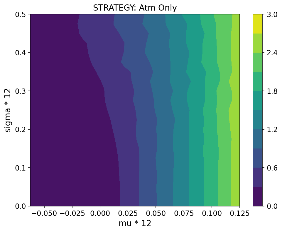
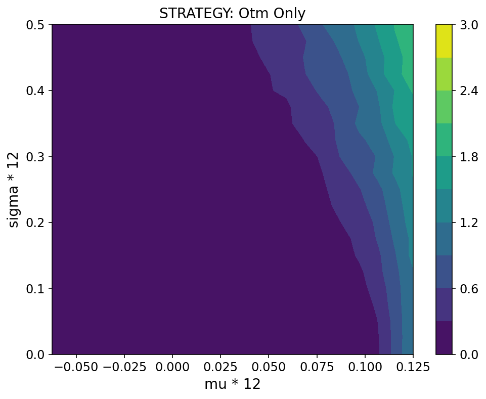
Leaving aside the subtle matter of converting between payouts and "utility", we can present the simulation results for a given allocation ruleset as a contour plot, with the two main parameters ($\mu$ and $\sigma$) on x- and y-axes and the payout as the third dimension (the color/contour level). As an example, the "cash only" ruleset leads to a flat plot with 0.9 for all values of the parameters, since the cash payout does not depend on the stock price. (Note: we are also ignoring effects of inflation here.). More interesting are plots for some of the other allocation rulesets (note: I have multiplied by $\mu$ and $\sigma$ by 12, which roughly converts them to annual quantities)
Allocation to RSUs only

Allocation to ATM options only

Allocation to OTM options only

We can draw a few conclusions:
- For the rates of return being simulated, the OTM options are strictly inferior to the ATM options. They become superior only for higher annual rates of return (>15%). This makes sense, given that the total appreciation over 4 years has to be >50% for these options to be worth anything, let alone better than the other equity types. (Using a longer time horizon, such as ten years, which is the typical expiration date for options, would change these conclusions.)
- RSUs are relatively unaffected by volatility ($\sigma$), but increased volatility actually helps options moderately. This is not too surprising, since options are a one-sided bet: you make money if the stock price goes up a lot, but don't lose money if it goes down a lot. So, for a low rate of return, increased volatility increases the likelihood of both the former outcome and the latter outcome, resulting in a higher expected payout.
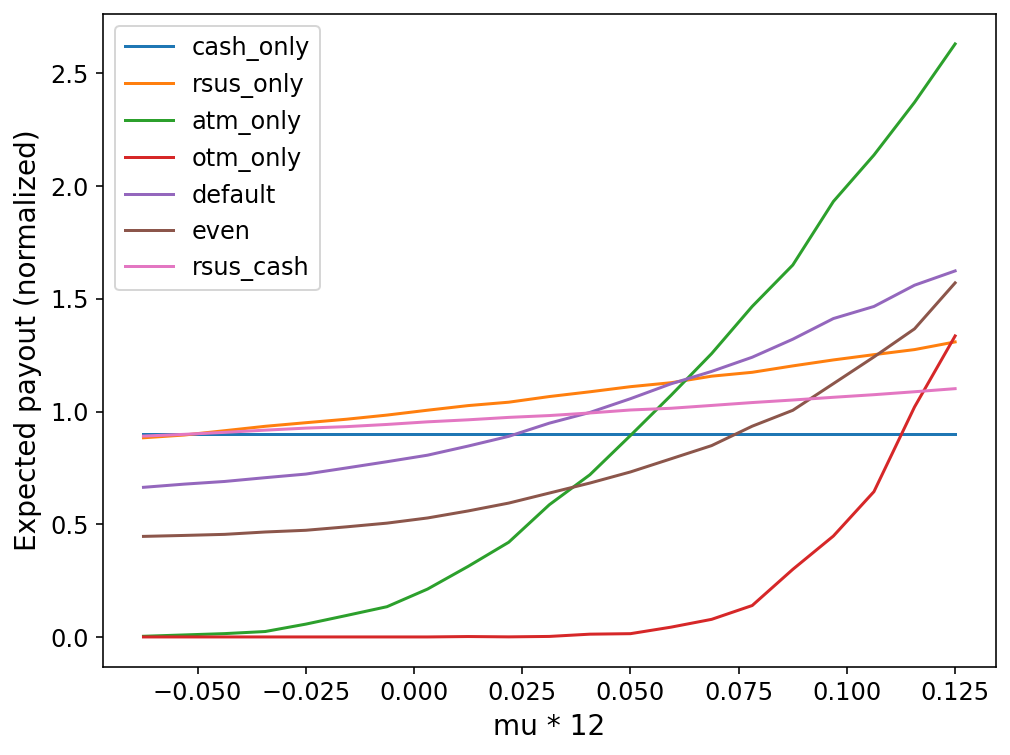
- Since the payouts are far more sensitive to $\mu$ than to $\sigma$, we can also plot these results in a more comprehensible line plot format, where we fix $\sigma$ (here, at $0.2/12$) and plot the results against $\mu$:

This plot provides a useful graphical summary of the different growth assumptions under which the various equity types make sense. It also shows how mixing options with RSUs and/or cash (the "default" and "even" allocations) can provide a compromise that still provides some payout under negative or low stock price growth, while providing substantial upside under high stock price growth.
Prior probabilities and utility functions
Arguably, the most difficult part of this exercise is not implementing the simulation, but generating a sensible prior distribution. Most tech stocks are very young, and therefore there may not be sufficient historical data to inform a prior. Moreover, assuming that future stock price movements will follow historical trends is always a dangerous assumption.
I don't have any great advice to provide here, but I think a wide Gaussian, centered at some positive rate of return that roughly equals the historical market return (say, S&P 500 or Nasdaq), seems reasonable. This choice avoids being overly optimistic, comprises a wide range of scenarios (negative, low, and high growth) and does not rely too heavily on thin historical data.
(Note: I am also only considering $\mu$ here. Estimating $\sigma$ is even more challenging, although, fortunately, it does not affect the results too much.)
The utility function is also highly subjective. In my case, I am fairly risk-averse, and therefore my utility function is shaped concave downwards (see here for examples). In contrast, others may view equity as "house money", and only care if they strike it rich and not care otherwise. This would be "risk-seeking" behavior. Ultimately, this is a personal decision that depends on your own financial situation and feelings towards money, and there is no single "right" answer.
It is also not obvious whether we should be looking at the expected value at all, particularly if we are risk averse. Perhaps we'd like to adopt a "maximin" approach, where we maximize the utility associated with a low-quantile outcome, such as the 10th or 25th percentile. This should be straightforward using the machinery we developed above, since we have effectively generated the entire payout probability distribution. The likely outcome, with respect to decision making, is that the optimal allocation shifts more towards cash/RSUs (safer assets) and away from options (riskier assets)
Summary and conclusions
To conclude:
- Monte Carlo simulations can be a powerful tool for decision making, when combined with a function that takes us from "outcomes" to "utility".
- These simulations have several interrelated pieces: a parametric equation describing how to move from time $t$ to $t+1$; a prior probability distribution for these parameters; and a ruleset followed by the actor (if relevant). By running simulations from the same initial conditions $N$ times, where $N$ is sufficiently large, we can generate the complete probability distribution for the simulation outcomes.
- We applied this framework to a specific problem: how to allocate equity across 4 different asset types to maximize the expected utility associated with the payout. Using a geometric Brownian motion model for the stock price, and some (slick?) Python code, we generated vaguely pretty plots that showed how payouts change with the volatility ($\sigma$) and the rate of return ($\mu$). Unsurprisingly, the four different asset types behave very differently in negative, low, and high growth regimes, and their behavior can be smoothed out by blending different asset types together.
- The most difficult part of this exercise lies in the subjective/unknowable aspects: the prior probability distributions and the utility functions.
- There were many dubious assumptions made (neglecting taxation, assuming a geometric Brownian motion model for stock prices, settling on a simple-to-code but suboptimal strategy for exercising options, etc.), so this should not be taken as a final word on this problem. Indeed, the purpose was more to show an example of the Monte Carlo simulation technique than to decide on an "optimal" allocation ruleset for me.
(For those who are curious, I plan to put the vast majority of my equity into RSUs; given my risk aversion, this decision makes more sense than the default allocation (75% RSUs, 25% ATM options), and RSUs are superior to cash even under somewhat pessimistic growth assumptions. That being said, I took the analysis above as more of a guide than anything else; I did not try to "argmax" my way to a decision.)
Addendum
The Jupyter notebook used to run the simulations, generate the plots, etc. is provided here