Against CUPED
Tl;dr
- CUPED is the most popular variance reduction technique in tech. It allows us to run shorter experiments without sacrificing power.
- It suffers, however, from several problems.
- It does not work on new “units” (e.g., users)
- Even for existing/tenured units, it does not work when the experiment tries to drive units from “0” to “1” (e.g., upgrading for the first time).
- It can mask problems with the metric itself. It’s better to first try simpler approaches (e.g., eliminating outliers, winsorizing, or binarizing) for reducing variance.
- It is flawed for binary metrics.
- It is also flawed in cases of imperfect randomization/pre-exposure bias
- While CUPED can be modified to address some of these deficiencies (”CUPED++”, etc.), such fixes often seem ad-hoc
- A better, cleaner approach is to use standard econometric techniques like regression or double ML to do variance reduction
Introduction
CUPED (”Controlled Experiments Utilizing Pre-Experiment Data”) is a technique for reducing variance when running A/B tests. For the same sample size, we get more power, or, for the same power, we need less sample size and can run shorter experiments.
CUPED is not just a variance reduction technique. It is by far the most popular variance reduction technique in tech. This fact is somewhat surprising for people coming from other fields, as Matteo Courthoud points out:
During my PhD, I spent a lot of time learning and applying causal inference methods to experimental and observational data. However, I was completely clueless when I first heard of CUPED (Controlled-Experiment using Pre-Experiment Data), a technique to increase the power of randomized controlled trials in A/B tests.
What really amazed me was the popularity of the algorithm in the industry. CUPED was first introduced by Microsoft researchers Deng, Xu, Kohavi, Walker (2013) and has been widely used in companies such as Netflix, Booking, Meta, Airbnb, TripAdvisor, DoorDash, Faire, and many others.
A few factors account for CUPED’s success.
- It is dead simple to implement. One of the posts linked above, by Simon Jackson at booking.com, shows how CUPED can be implemented in SQL alone. This means CUPED can scale to data that doesn’t fit in memory, unlike some Python-based (e.g., ML) variance reduction techniques.
- It provides decent results without too much “fiddling” or parameter tuning. (CUPED basically has only one free parameter, the lookback window for the pre-experiment metric). CUPED never increases the metric variance, and, in practice, it can decrease the required sample size for an experiment by 20% or more. Because it makes a linear adjustment, it basically never overfits, unlike some ML-based techniques.
- It is widely available in commercially available platforms for experiment analysis, such as GrowthBook, StatSig, and Eppo. With the exception of Eppo, it appears to be the only variance reduction technique offered by these platforms, at the time of this writing.
- Perhaps most importantly, it came out of Microsoft, and is part of the industry-standard “Hippo book” (”Trustworthy Online Controlled Experiments”). If it’s good enough for Microsoft’s experimentation platform, it’s probably good enough for your company’s.
I find CUPED useful for my own work, on occasion. That being said, it has some serious limitations, and, below, I present 5 critiques of CUPED. In order, they are:
- CUPED does not work on new “units” (e.g., users)
- Even for existing/tenured units, CUPED does not work when the experiment is designed to encourage these units to do something for the first time, like upgrade.
- Some of the problems CUPED addresses can be mitigated by modifying the metric itself (e.g., eliminating outliers, winsorizing, or binarizing). Some of the estimates of “increase in effective sample size” are misleading or exaggerated because they compare CUPED to nothing at all, as opposed to these other tactics.
- CUPED, at least in its naive implementation, should probably not be used for binary metrics.
- Naive CUPED also does not fix imperfect randomization/pre-exposure bias. The non-naive implementation, which does correct for pre-exposure bias, isn’t well-known.
Most practitioners are aware of at least some of these problems (in particular, 1 and 2), but I have not seen all of them presented in a single place before.
I’ll also provide some code examples to allow readers to follow along more easily. Let’s go!
A basic CUPED example
Assume a standard, two-cell A/B test. The primary metric is continuous — say, streaming time, on a platform like Spotify. We’re experimenting on tenured users who have enough data for this metric before the experiment begins.
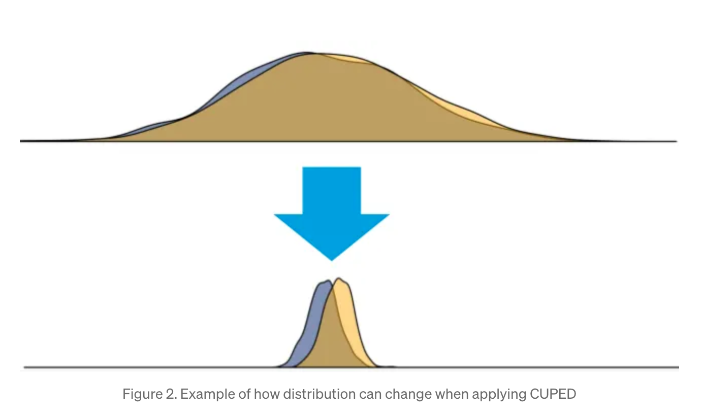
The great insight of CUPED is that the metric of interest is often correlated with its pre-experiment value. Users who stream for longer before the experiment should also stream longer during the experiment. In fact, much of the variance in streaming time is due to the heterogeneity in users, and, by eliminating this factor, our estimates of the effect size become much more precise (smaller standard error). Simon Jackson has a nice graphic, reprinted below. You can see that it would be much easier to measure the treatment effect in the second image than in the first image.
Let’s write some code! (Much of this is adapted from Matteo Courthoud’s excellent blog post about CUPED.) See here for the complete code, including a Jupyter notebook.
In the data generation process, the continuous metric, $y$, is linearly related to the experiment group assignment (control = 0, treatment = 1), and to the pre-experiment value of $y$, which we'll call $X$. There is also Gaussian noise. The treatment effect is constant across all units (no heterogeneous treatment effects).
$X$, in turn, might also be related to the experiment group assignment, if we have imperfect randomization/pre-exposure bias. (In this case, users in treatment stream for longer than users in control, even before the experiment begins.)
# adapted from https://github.com/matteocourthoud/Blog-Posts/blob/9b5ff8276b8a197ccbbe97fa1e26f3e87871544d/notebooks/src/dgp_collection.py
class DataGenerationContinuousMetric:
    def __init__(
        self,
        y0_intercept=5,
        y0_bias=0,
        y1_offset=3,
        treatment_effect=0.1,
    ):
        self.y0_intercept = y0_intercept
        self.y0_bias = y0_bias
        self.y1_offset = y1_offset
        self.treatment_effect = treatment_effect

    def generate_data(self, N=10000, seed=1):
        rng = np.random.default_rng(seed)

        # Individuals
        i = range(N)

        # Treatment status (0 = control, 1 = treatment)
        experiment_group = rng.choice(a=[0, 1], size=N)

        # Pre-treatment value of metric (Gaussian)
        y0_noise = rng.normal(loc=0.0, scale=1.0, size=N)
        y0 = self.y0_intercept + self.y0_bias * experiment_group + y0_noise

        # Metric (linearly related to pre-treatment value of metric)
        y1_noise = rng.normal(loc=0.0, scale=1.0, size=N)
        y1 = y0 + self.y1_offset + self.treatment_effect * experiment_group + y1_noise

        # Generate the dataframe
        # use y0 (pre-treatment value of metric) as the covariate, X
        # rename y1 to y
        df = pd.DataFrame(
            {"i": i, "experiment_group": experiment_group, "X": y0, "y": y1}
        )

        return df
When we run generate_data, we’ll create a DataFrame of N rows, one for each user. Our goal is to estimate the true treatment effect with as little variance as possible (small standard error). To avoid having to derive the standard error analytically, we’ll simply run a lot of simulations with different seed values, and compute the standard deviation manually, Monte Carlo style.
Here’s a simulation routine (again, adapted from Matteo Courthoud’s blog post):
def simulate(dgp, estimators, N_trials=1000, sample_size=10000):
    results = []

    # Conduct N trials, generating new data for each one
    for trial_num in range(N_trials):
        # Draw data
        df = dgp.generate_data(seed=trial_num, N=sample_size)

        # Iterate over estimators, generating estimate for each
        for estimator, estimator_func in estimators:
            estimate = estimator_func(df)
            result = {
                "trial_num": trial_num,
                "estimator": estimator,
                "effect_size": estimate
            }
            results.append(result)

    return pd.DataFrame(results)
We supply the estimators, which are functions that take the dataframe and return the treatment effect estimate. Below are the first two estimators we’ll focus on: the “naive” estimate, which is what a simple t-test would give you, and the "CUPED” estimate, which uses the pre-experiment data, X, to reduce the variance of y.
def naive(df):
    estimate = smf.ols('y ~ experiment_group', data=df).fit().params.iloc[1]
    return estimate

def cuped(df):
    df = df.copy()
    df['y_tilde'] = smf.ols('y ~ X', data=df).fit().resid + np.mean(df['X'])
    estimate = smf.ols('y_tilde ~ experiment_group', data=df).fit().params.iloc[1]
    return estimate
Let’s verify that CUPED actually works!
dgp = DataGenerationContinuousMetric(treatment_effect=0.1, y0_bias=0)
estimators = [
    ("naive", naive),
    ("cuped", cuped),
]
results_frame = simulate(dgp, estimators=estimators, N_trials=500, sample_size=10000)
(
    results_frame
    .groupby(by=["estimator"])
    .agg(
        treatment_effect_mean=("effect_size", "mean"),
        treatment_effect_std=("effect_size", "std")
    )
)
When I run this, I get:
| estimator | effect_size_mean | effect_size_std |
|---|---|---|
| cuped | 0.099907 | 0.019107 |
| naive | 0.099947 | 0.026958 |
And, in visual form:
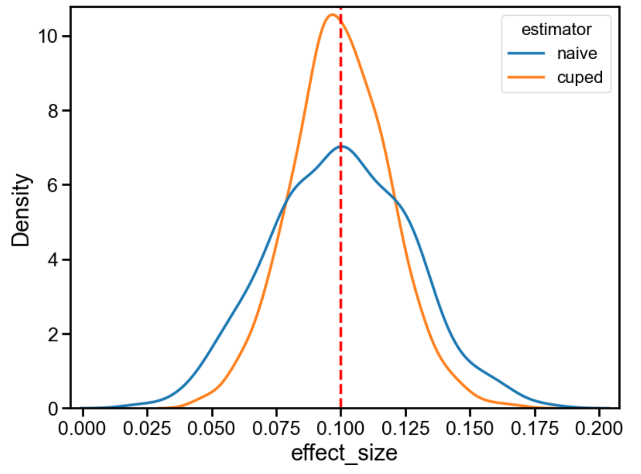
As expected, both techniques recover the correct treatment effect (0.1). CUPED has a much smaller standard deviation, though (roughly, 0.0191/0.027 = 71%). This means that, in this synthetic example, we can run this test for 1 - 0.71^2 = 50% less time with CUPED, and get the same statistical power. Cool!
5 problems with CUPED
Now comes the part where I explain why, disappointingly, the previous example is basically as rosy as it gets. In practice, CUPED can be much less effective, or completely ineffective. I don’t want to discount cases where it works well. But, at least in my current work, those are few and far between.
Problem 1: New units
CUPED relies on the existence of pre-experiment data for the metric of interest. But what if we’re targeting new units, for which such data doesn’t exist?
Suppose we want to drive streaming time for new users on Spotify. The “pre-experiment” metric is 0 — these units don’t have any streaming time before they are exposed to the experiment, since they weren’t Spotify users then.
As Eppo explains,
The standard CUPED approach does not help for experiments where no pre-experiment data exists (e.g. experiments on new users, such as onboarding flows).”
Because we also use assignment properties as covariates in the regression adjustments model, we are able to reduce variance for these experiments as well, which leads to smaller confidence intervals for such experiments.
Put differently: one problem with CUPED is that, in the typical implementation, we use the pre-experiment metric to adjust the experiment metric. But this approach is part of a larger class of “covariate adjustment” methods for reducing variance. We don’t have to use the pre-experiment metric as the sole covariate. We can use any number of covariates that are known at exposure time or before.
For new users on Spotify, we might know their device, country, or acquisition source, and we might be able to infer other characteristics, like age and gender. To the extent that these are correlated with streaming time, they can help reduce variance. Eppo has termed this approach “CUPED++”, but, in my view, this isn’t really CUPED anymore.
Unfortunately, in my experience, “demographic” covariates like country — as opposed to “usage-based” covariates, like the pre-experiment value of the metric — tend to be weak predictors of usage metrics. The efficacy of CUPED, and other variance reduction techniques, is basically proportional to this predictive power ($R^2$, roughly speaking). So, if assignment-time covariates are only weakly correlated with the metric of interest, as they typically are for new units, then the gains from variance reduction will be correspondingly small.
When employing variance reduction, it’s important to ask: how much of the heterogeneity in the metric can be explained by covariates (whether the pre-experiment metric, or others)? If the answer is “not much”, CUPED, or even “CUPED++”, is not likely to be effective.
Problem 2: Getting existing units to do something for the first time
Product development, especially at smaller companies, often focuses on getting “units” to do something for the first time, regardless of how long they’ve been tenured. We want tenured free users, who have been freeloading for years, to pay for the first time. We want paid teams to upgrade to a higher plan type. We want users to stream a playlist they haven’t listened to before, or try our new group listening feature, or peruse their first audiobook. The first step in establishing a habit with a feature is trying it once. That’s also often the hardest step.
So, typically, the primary metric in an experiment will be some version of what I discussed above. Whether a user paid. Whether a team upgraded. How long a particular playlist was listened to. Group listening session time. Audiobook consumption. Etc.
The problem is that the pre-experiment metric is 0 for users who haven’t done those things before. An experiment designed to get free users to pay will not benefit from CUPED! That’s true even if these users aren’t new users. In the case where the targeted population is a mix of users — some of whom have done the target action before, some who haven't — CUPED is more ineffective the larger the latter group becomes relative to the former.
CUPED came out of Microsoft, where much of the product development is incremental, not greenfield. In these cases, CUPED is more likely to be successful. Say we’re trying to increase search success of Bing, or trying to reduce error rates with Microsoft Office. It seems likely that some (much?) of the heterogeneity in these metrics is at the user level. (For instance, users with worse devices are more likely to have errors.) Sadly, this kind of experimentation isn’t representative of that at many tech companies.
It isn’t even representative of other teams at Microsoft! In a post from 2022 (many years after the advent of CUPED), Microsoft’s experimentation platform team reported on the success rate of CUPED for different teams (”product surfaces”) at Microsoft. They found:
…[a] substantial difference in efficacy across different product surfaces and metric types.
Based on a recent 12-week sample of week-long experiments, groups of VR [Variance Reduction] metrics from two different surfaces for the same product have very different average performance. In one Microsoft product surface, VR is not effective for most metrics: a majority of metrics (>68%) have effective traffic multiplier <=1.05x. In contrast, another product surface sees substantial gain from VR methods: a majority of metrics (>55%) have effective traffic multiplier >1.2x.
Before investing heavily into CUPED or other variance reduction techniques, you should try to figure out if your “product surface” is more like example 1 or example 2.
Problem 3: CUPED might mask a underlying metric problem
I’ve always been slightly peeved by the toy examples used to demonstrate the power of CUPED. They employ nice and neat Gaussian distributions. In practice, things aren’t so simple!
Before using CUPED, or other variance reduction techniques, it’s worth asking: why is the metric high-variance to begin with? Some possible explanations:
- The metric has bad values. Some users stream for more than 24 hours in a day. (E.g., they are bots, or are running a scheme like this one.) It’s better to clean up bad values than to paper over them with CUPED.
- The metric has (valid) outliers. Some companies contribute disproportionate revenue to your SaaS business. Some people have unusually laggy devices. CUPED might help, marginally, in these cases, but it would involve a regression that is unduly influenced by “high-leverage” observations. A better approach would be to winsorize these outliers, or to use a regression robust to outliers, like quantile regression.
- The metric doesn’t have outliers, but is very right-tailed/skewed. Such distributions abound in tech. Most people are around 400-1000 Elo on chess.com, but some are 2500+. Many people stream Taylor Swift a little bit, but some are superfans. Some artists, like Bad Bunny or The Weeknd, receive orders of magnitude more streams, and payouts, than the median artist. Once again, winsorization can be a useful approach here. Or quantile regression. Or turning the continuous metric into a binary one. (At Spotify, we used to have a metric called “deep listens”, which meant a user had more than 15 streams from a particular playlist. It was a binary version of a continuous metric: playlist streams.)
All of these approaches — winsorization, outlier removal, binarizing a continuous metric — squeeze variance out of the original metric. It makes sense, then, that subsequent “squeezing” would be less effective: the winsorized or binarized metric would benefit much less from CUPED or other variance reduction techniques than the original metric. Let’s try to prove this!
Suppose the pre-treatment covariate, $X$, comes from a lognormal distribution, instead of a Gaussian one (this causes the distribution of both $X$ and $y$ to be right-tailed):
# (in the __init__ function for the data generating process class)
if self.y0_noise_dist == "normal":
    y0_noise = rng.normal(loc=0.0, scale=1.0, size=N)
elif self.y0_noise_dist == "lognormal":
    y0_noise = rng.lognormal(mean=0.0, sigma=1.0, size=N)
Then, winsorize or binarize the metric as follows:
# apply winsorization/binarization (optional)
if winsorize_q is not None:
    cutpoint = df["y"].quantile(winsorize_q)
    df = df.assign(
        y=lambda df: df["y"].clip(upper=cutpoint),
    )
elif binarize_q is not None:
    cutpoint = df["y"].quantile(binarize_q)
    df = df.assign(
        y=lambda df: (df["y"] > cutpoint).astype(int),
    )
We can repeat the original simulation, two times. In the first, we winsorize at the 95th percentile. In the second, we binarize at the 50th percentile. We find (see notebook):
| Dataset | Variance Reduction (%) | z-score (Naive) | z-score (CUPED) |
|---|---|---|---|
| original | 83% | 2.16 | 5.23 |
| winsorized | 47% | 2.95 | 4.07 |
| binarized | 16% | 2.88 | 3.14 |
One important note: because of the way this simulation was constructed — homogeneous treatment effect, strongly linear relationship between pre-treatment covariate and metric, etc. — the CUPED-adjusted, non-winsorized metric still performs the best. It has the highest “z-score” and, of course, winsorization or binarization change the metric being measured, so we can’t expect to recover the original effect size (see code/notebook).
However, note that winsorized and binarized metrics are more sensitive than the original metric (without CUPED). The z-scores are higher, and it's easier to detect an effect. I'd recommending trying such approaches before investing in variance reduction.
Another important point is that the benefits of CUPED are often overstated. If you do nothing to your continuous metric, CUPED can yield very large variance reduction (here, >80%). But usually you’ll use winsorization, outlier removal, or binarization, and in these cases the benefits from variance reduction are often much smaller. “Truncating” metrics is standard practice in tech. So why do proponents of CUPED act as if it’s not?
(Side note: the CUPED results I reported on for the truncated metrics is not exactly CUPED. The metric is truncated, but the pre-experiment value is not. That is, we're not using the exact same metric as the pre-experiment covariate.
It turns out that CUPED works less well if the pre-experiment value is also truncated. Again, this points to the need to investigate a variety of covariates, not just the pre-experiment value.)
Problem 4: CUPED shouldn’t be used for binary metrics
I used CUPED above for binary metrics, and it did reduce variance. Strictly speaking, though, it is inappropriate in this case! (Optimizely, for example, uses CUPED only for continuous metrics.)
When doing covariate adjustment, we should subtract off $E[y|X]$ from $y$. The problem with CUPED is its estimate of $E[y|X]$ is wrong, since it uses a linear model for a binary target. Instead, we should use a logistic (or similar) model instead.
Again, looking at a simulation is helpful. Let’s use the following CUPED-like estimator for binary metrics:
def cuped_binary(df):
    df = df.copy()
    df["y_tilde"] = smf.logit("y ~ X", data=df).fit(disp=0).resid_response
    estimate = smf.ols("y_tilde ~ experiment_group", data=df).fit().params.iloc[1]
    return estimate
(Note the logit instead of ols for the “first-stage” regression.)
Run the usual simulation:
dgp = utils.DataGenerationContinuousMetric(
    treatment_effect=0.1,
    y0_noise_dist="lognormal"
)
estimators = [
    ("naive", utils.naive),
    ("CUPED", utils.cuped),
    ("CUPED binary", utils.cuped_binary),
]
results_frame_binarize = utils.simulate(
    dgp,
    estimators=estimators,
    N_trials=1000,
    sample_size=10000,
    binarize_q=0.5,
)
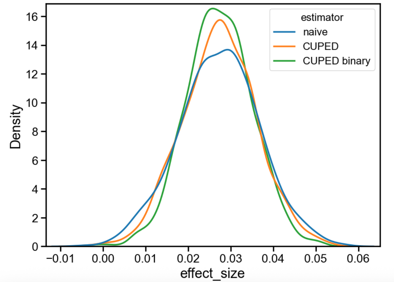
Although the differences might look small, the “CUPED binary” estimator is clearly the best. It provides the tightest estimate of the true effect. In this case (see notebook), while ordinary CUPED yields a 16% variance reduction, the binary CUPED approach achieves 33% variance reduction. Not bad for a relatively simple fix!
Problem 5: CUPED doesn’t fix pre-exposure bias
Pre-exposure bias is a common problem in experimentation. The treatment and control groups will never exactly agree in every important covariate, particularly when the distributions of those covariates are skewed. It is possible, by chance, to end up with more users with higher $X$ values in treatment. Some experimentation platforms try to weed out “bad randomization seeds” (see here for Microsoft's approach), but many do not. Instead they use covariate adjustment techniques, like CUPED, to mitigate the bias after the fact.
But does CUPED actually correct for pre-exposure bias? It seems like it should. After all, the bias is from the covariate, $X$, being imbalanced, and we’re basically trying to subtract out its effect. As it turns out, though, CUPED doesn’t totally solve the problem. Here’s an example (again, adapted from Matteo Courthoud’s blog post, with an artificially large treatment effect of 1 to clearly show the problem):
dgp = DataGenerationContinuousMetric(
    treatment_effect=1, y0_bias=1
)
estimators = [
    ("naive", naive),
    ("CUPED", cuped),
]
results_frame = utils.simulate(
    dgp,
    estimators=estimators,
    N_trials=1000,
    sample_size=10000
)
(
    results_frame
    .groupby(by=["estimator"])
    .agg(mean=("effect_size", "mean"), stddev=("effect_size", "std"))
)
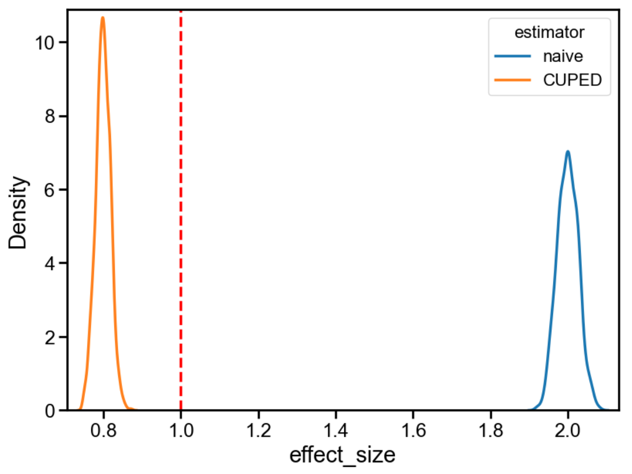
The true effect is 1. The naive estimate is 2 (because the bias we induced is an extra 1). CUPED, however, returns 0.8, which is neither 1 nor 2: it overcorrects in the opposite direction.
This result is surprising if you believe statements like this (from Statsig):
CUPED (short for Controlled-experiment Using Pre-Existing Data) is a technique which leverages user information from before an experiment to reduce the variance, and increase confidence in experimental metrics. This can help to debias experiments which have meaningful pre-exposure bias (e.g. the groups were randomly different before any treatment was applied).
What’s going on here? It turns out that the naive implementation of CUPED — e.g., from the original paper, or from Simon Jackson’s blogpost — assumes perfect randomization. A more recent implementation, from this Microsoft blogpost, fixes this problem (oddly, without acknowledging it is a problem).
See code below:
def cuped_advanced(df):
    df_treatment = df.query("experiment_group == 1")
    df_control = df.query("experiment_group == 0")
    p_treatment = df_treatment.shape[0] / df.shape[0]
    p_control = df_control.shape[0] / df.shape[0]
    theta_treatment = smf.ols('y ~ X', data=df_treatment).fit().params.iloc[1]
    theta_control = smf.ols('y ~ X', data=df_control).fit().params.iloc[1]
    theta_avg = p_control*theta_control + p_treatment*theta_treatment
    y_tilde_avg_treatment = df_treatment.assign(
        y_tilde=lambda df: df["y"] - theta_avg * df["X"]
    )["y_tilde"].mean()
    y_tilde_avg_control = df_control.assign(
        y_tilde=lambda df: df["y"] - theta_avg * df["X"]
    )["y_tilde"].mean()
    estimate = y_tilde_avg_treatment - y_tilde_avg_control
    return estimate
When we rerun the simulation, we see that “advanced CUPED” does indeed recover the correct treatment effect, even when pre-exposure bias is a problem.
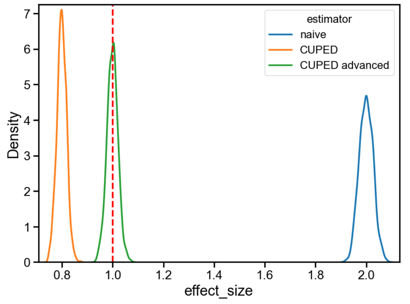
As far as I can tell, though, most people (even Statsig, possibly?) are apparently unaware of this issue. So, word to the wise: be careful when implementing CUPED, and use cuped_advanced instead of cuped if pre-exposure bias is expected to be a problem.
(Side note: as you can see, “simple CUPED” actually does have a smaller standard error than “advanced CUPED”, even though the estimate is biased. There is no free lunch here: the estimator that works better in the presence of pre-exposure bias is not the estimator that works best if we can assume away that bias.)
Summary and closing thoughts
Variance reduction is as close as we get to a free lunch in experimentation. Without sacrificing power, we can run shorter tests and gain insights faster. But variance reduction is not always useful, and CUPED, in particular, suffers from several problems.
CUPED uses the pre-experiment value of the metric as the sole covariate. It doesn’t work when this value doesn’t exist (as with new users), or when it’s zero (as with existing users being encouraged to do something for the first time, such as purchase). In these situations, it’s better to use “assignment-time covariates” (”CUPED++”) rather than CUPED, but don’t expect much variance reduction unless these covariates are well-correlated with the metric — which, in my experience, is usually not the case.
The value of variance reduction techniques is often demonstrated in examples involving continuous metrics. Such metrics may intrinsically have high variance, but this variance can be reduced by outlier removal, winsorization, binarization, and other techniques. (This also generally improves metric sensitivity.) After truncating the metric, CUPED helps much less. We’ve squeezed out some of the variance, so CUPED has less left to further squeeze. It’s worth trying these (easy-to-implement) techniques before investing in variance reduction. And you should be wary of taking estimates of variance reduction at face value.
“Simple CUPED” also just isn’t correct in some cases. It can be improved for binary metrics by using logistic instead of linear regression for the “first stage”. And, surprisingly, it also doesn't totally fix pre-exposure bias, and "advanced CUPED" should be used instead.
I found it somewhat unsatisfying to learn that CUPED requires these ad-hoc adjustments. Is there a less arbitrary approach to variance reduction?
In fact, there is! "Advanced CUPED" is equivalent to a “fully-interacted” linear regression model, ANCOVA2. See code below. And using a classifier, not a regressor, for binary metrics to use logistic regression is what packages like EconML do by default for discrete outcomes.
def ancova2(df):
    # optional step, makes coefficients more interpretable
    X_mean = df["X"].mean()
    df = df.copy().assign(X_demeaned=lambda df: df["X"] - X_mean)
    estimate = (
        smf.ols(
            "y ~ experiment_group + X_demeaned + experiment_group * X_demeaned", data=df
        )
        .fit()
        .params.iloc[1]
    )
    return estimate
If there’s a lesson here, it’s that we should use standard econometric techniques instead of ad-hoc adjustments like CUPED. In fact, every example in this post can be re-done using “double machine learning” models in EconML with (generalized) linear first and second stages. (I’ll demonstrate this in a subsequent blogpost!)
(Side note: some people mistakenly assume that naive CUPED is equivalent to a regression like $y \sim X + T$. See Matteo Courthoud's blogpost for a demonstration that this isn't true.)
Double ML models have a number of benefits over CUPED. They work for binary or continuous outcomes, and binary or continuous treatments. They can account for any number of covariates, not just the pre-experiment metric. They also work for experimental and observational data — e.g., when treatment and control aren’t balanced, and there is selection bias. They can even capture heterogeneous treatment effects and non-linear relationships in the data (although these applications tend to be data-greedy). Most importantly, they tend to have good numerical properties, and are less sensitive to incorrect estimates of nuisance parameters ("Neyman orthogonality")
Double ML models are not easy to implement in SQL, even when the individual stages are linear. There’s a reason CUPED is still king: data scientists are lazy, and we’ll go with the “good enough” option if it’s much easier to code. But this dilemma seems artificial to me. I’d hope that commercial platforms would do the hard work of implementing the correct solution so we wouldn’t have to choose.