Trending towards significance, revisited

Tl;dr

• I discuss whether a marginal p-value (one “bordering” on statistical significance) can be accurately characterized as “trending towards” significance.
  • This would imply that, if we ran the experiment for longer, we would (eventually) see significance
• One explanation provided — that p-values exhibit no average trends, because the t-statistic is a zero-mean random walk — is, at best, incomplete.
• There are trends in p-values, but these trends are sensitive to the prior distribution, which we can’t accurately know.
• So, we should not make statements akin to “trending towards significance”, although for different reasons than have been stated elsewhere.

Introduction

Product managers often want to salvage an experiment that failed to find statistical significance. They might claim that, although the primary metric was not statistically significant, it “verged” on significance, or was “trending towards” significance. Are these claims statistically valid?

Let’s make precise the notion of “trending towards statistical significance”. Here is an explanation from a scientific paper, "Trap of trends to statistical significance: likelihood of near significant P value becoming more significant with extra data” by Wood et al.

When faced with a P value that has failed to reach some specific threshold (generally p<0.05), authors of scientific articles may imply a “trend towards statistical significance” or otherwise suggest that the failure to achieve statistical significance was due to insufficient data.

…

Instead of reporting trends, some authors imply that their results got close to or bordered on significance. Quite elaborate forms of words may be used, such as “teetering on the brink of significance.” They imply that, with a nudge (extra data), significance would plausibly have been achieved.

In other words, if we had run the experiment longer, we would have observed significance. The fault lies not in the efficacy of the treatment — the quality of the idea —, but instead in our inadequate sample size. Such an explanation is obviously self-serving — no one wants to admit their ideas don’t work — but is it also wrong?

In the paper mentioned above, the authors conduct a numerical simulation showing that “trending towards significance” is statistically invalid. In my view, though, this exercise doesn't provide much intuition for why this is the case.

A recent post by Zach Flynn purports to provide a simple explanation. He writes

You may have heard that the result of an experiment is “trending” towards significance despite currently being insignificant. It isn’t. But the reason why is difficult to find by Googling. This short post is my attempt to put the info out there!

For a math-free intuition of the main point, suppose it was possible to predict whether a currently insignificant result was “trending” towards becoming significant. Wouldn’t this make the result significant today? i.e., if you could tell, based on current information, whether the result would be significant in the future, it would be significant now!

…

A little more precisely: W(n) [the t-statistic as a function of sample size, n] is a random walk. For large n, W(n) is approximately a Weiner process, and increments in a Weiner process are independent of their historical values.

The purpose of this essay is to explore this set of claims, using numerical simulations (and some theory). I find, contrary to Zach, that:

• The assumptions that make the t-statistic a random walk are not necessarily applicable to the A/B tests we care about. Specifically:
  • The assumption about (additional) sample size
  • The assumption about the treatment effect
• We don’t just care whether changes in the t-statistic are independent of their historical values. We also care whether these changes are, on average, zero or non-zero: does the t-statistic grow over time?
• If the null hypothesis is true, changes in the t-statistic are negatively correlated to the current value of t. This is a form of mean reversion/”regression to the mean”.
• On the other hand, if the alternative hypothesis is true, changes in the t-statistic are still negative correlated to the current value of t, but, on average, t grows over time. In this case, perhaps not surprisingly, we really just do need more sample to see significance.
• The real problem with making statements like “trending towards significance” is that we don’t know, a priori, how likely the null or alternative hypothesis is. Is it simply random noise that will attenuate over time, or real signal that will grow with more observations?
• Therefore, it’s still good advice to caution PMs from using this kind of language.

Simulation approach

Let’s consider the following “trial” of a Monte Carlo simulation:

1. We compute the sample size required to measure a particular “detectable effect” with $\alpha =0.05$ and power = 0.8
   • The effect can either be 0 (null hypothesis) or the detectable effect (alternative hypothesis)
2. We draw samples for control and treatment, using the mean (for control) or mean + effect (for treatment), and a common variance (here, treatment effect/variance = 0.05)
3. We compute the following t-statistics and p-values:
   • "Underpowered": with sample size equaling only 50% of the exposures needed for power
   • "Slightly more": with slightly more (51%) of the required exposures (2% more in relative terms)
   • "Well powered": with all of the required exposures; 100% more in relative terms

We do this $N_{trials}$ times, Monte Carlo style. The setup is similar to the situation mentioned above, in which a PM might claim a result is insignificant due to lack of sample size. Here we simulate what would happen if we could run the test for slightly longer (”slightly more”) or much longer (”well powered”).

Code can be found in this Colab notebook. The figures reproduced below depict the correlations between the t-statistic at “a” (halfway through) and the change in the t-statistic with additional sample size (either "slightly more" or "well powered"). We want to determine two things.

1. Is the change in the t-statistic, on average, non-zero?
2. Is it correlated with the t-statistic itself?

Only if both of the answers are “no” do we get a (zero-mean) random walk. And, if the process is not a zero-mean random walk, then the t-statistic and p-value might be trending towards, or away from, significance.

Analysis

Null hypothesis

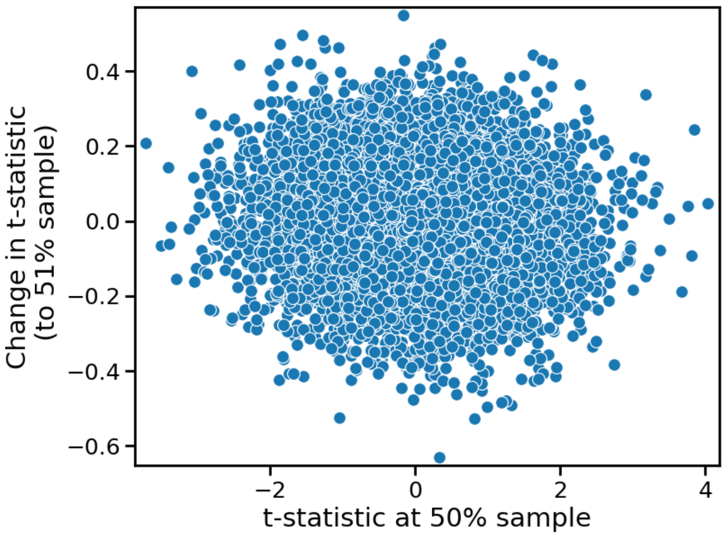
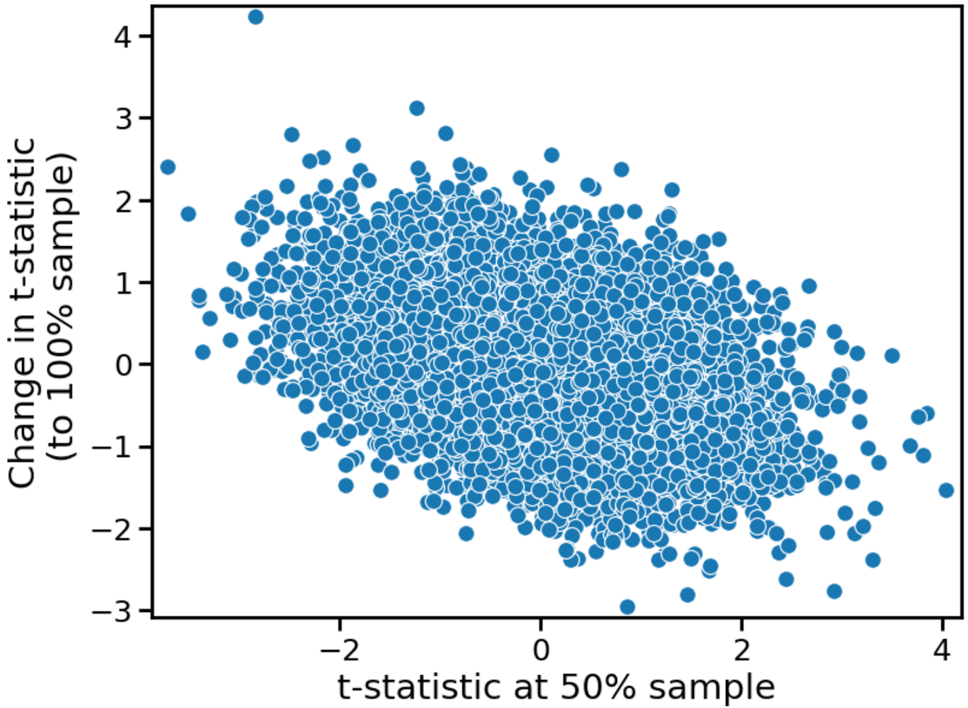
For the null hypothesis, we get the following two figures (first for 51% sample, second for 100% sample)

It is true, as Zach Flynn wrote, that for slightly more sample, the change in the t-statistic is uncorrelated with the t-statistic itself. Moreover, this change is on average zero: not surprising, given that the null hypothesis is true. So, if we run an A/B test for slightly longer, and there is no effect, the p-value will go up with 50% probability, and down with 50% probability. In this scenario, “trending towards significance” is meaningless, because there is no trend.

Let's now turn to the "well powered" case. For much larger sample, the average change remains zero, but the slope of the data is negative. Higher initial values of t produce lower final values of t. We have “mean reversion” or “regression to the mean”. Why might this be happening?

(Note: We can see this phenomenon even in Zach’s original derivation. He took the zeroth order expansion about "m" (the additional sample size), but the first order expansion has a negative coefficient.)

To gain intuition, consider the case of flipping a coin. We know that coin flips in the future are uncorrelated with coin flips in the past, and, therefore, the change in "heads minus tails" should be independent of the current value of this metric. We also know that the change in this metric should be zero in expectation, assuming a fair coin. This is a classical zero-mean random walk.

However, the change in “% heads” is not a random walk. While the absolute metric meanders randomly, the percentage metric converges towards 50%, in the long run. Values that initially deviate from 50%, because of randomness, eventually revert, even if the absolute metric does not. The division by “n” (the number of flips, or sample size) exerts a damping influence.

In our case, we have a similar damping influence, although it’s $1/\sqrt{n}$, because of the standard error, not $1/n$. For small additional sample size, we get the zero-mean random walk, but for larger additional sample size, we witness mean reversion. Large positive values of t decline over time, and large negative values of t increase over time. If the null hypothesis is true, everything is non-significant in the long run.

Alternative hypothesis

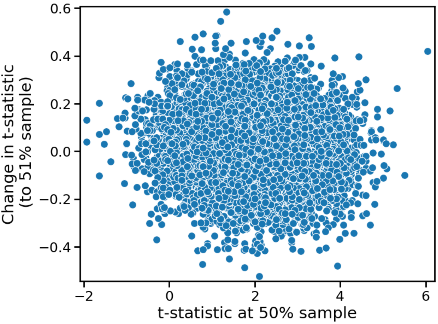
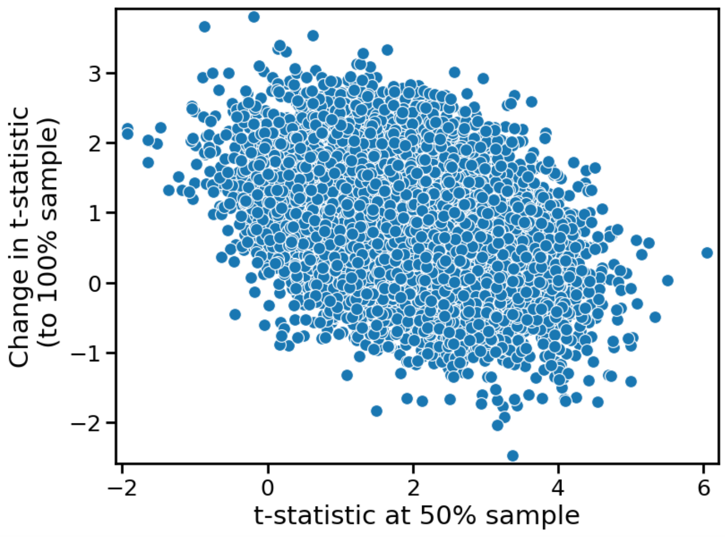
Corresponding figures are presented below for the alternative hypothesis.

The shape of the distribution remains the same, but the y-values — the growth in the t-statistic — are offset from zero. Since the treatment effect is non-zero, the average t-statistic grows over time. This is true even for the marginal values of t (just below $t_{crit}$) for which we might want to claim a “trend towards significance”.

In this case, we genuinely see a "trend towards significance”. If there is a real treatment effect, then we simply need to run the test longer, collecting more sample size, to observe a statistically significant effect. At only 50% sample size, we are underpowered. At 100% sample size, we are powered to 80%. For an even larger sample, we can achieve correspondingly larger values of power. And, in the limit of infinite sample size, we have 100% power, and are therefore guaranteed to observe a statistically significant effect.

The real problem with “trending towards significance”

The real problem with “trending towards significance” is not that p-values and t-statistics don’t exhibit trends — they clearly do. The problem is that these trends are highly sensitive to the true treatment effect. If we knew the exact weights or probabilities of the null and alternative hypothesis, or the prior distribution for the effect size, we could determine if the trend would be (on average) favorable or unfavorable. But, of course, we don’t.

We can take values commonly assumed in the literature, where $p_{null}$ is large: 85% or 90%. (This reflects the fact that most experiments have null effects.) Under this assumption, any trend towards significance is likely small, since the effect of the null hypothesis predominates. (The trend is also highly sensitive to the magnitude of the effect assumed in the alternative hypothesis.) These phenomena can be explored numerically, in the Colab notebook, by using different values for w_null and effect_size. Is this exercise useful? Probably not: we cannot reliably estimate these values a priori, and, even if we could, it wouldn’t translate into practical advice for PMs and others.

Conclusion

“Trending towards significance” is a self-serving phrase used to justify or salvage failed experiments. We’d like to believe the fault is in our stars, not in ourselves; that our sample size was inadequate, not our ideas. But that doesn't necessarily mean "trending towards significance" is also self-serving! Some of the attempted debunkings of “trending towards significance” seem, to me at least, to be bogus or unhelpful. t-statistics are not zero-mean random walks, and they do, in fact, exhibit trends.

If the null hypothesis is true, the trend is “mean reversion”. Large t-statistics (in magnitude) attenuate with additional sample size, as the initial randomness gets washed out. This trend is the opposite of what we’d like in order to justify a marginal p-value being statistically meaningful.

If the alternative hypothesis is true, however, the trend is growth, on average. Because an effect truly does exist, t-statistics trend towards significance with additional sample size. This is not surprising given that more sample size guarantees more power. In this case, saying “trending towards significance” is indeed acceptable.

The real problem is we don’t know, a priori, which of these situations has manifested. Are we observing a marginal p-value because of noise that will cause the t-statistic to diminish over time, or because of signal that will cause it to grow, secularly? We simply don’t know. Even if we did know, any statement we could make would be probabilistic (depending on the prior distribution of the effect size), not deterministic. To ascertain what would actually happen requires more sample size, and, if we had that sample size, why wouldn’t we just run the test longer instead of guessing?

(This finding echoes several of my previous posts on the “prior sensitivity” of A/B testing. See here, here, and here if interested.)

One last point: a marginal p-value isn’t useless. It provides weak evidence, not zero evidence. I liked this quote from the Wood et al. paper:

Overall, we would like to see greater recognition that individual P values in the region of 0.05 represent quite modest degrees of evidence, whichever side of the divide they lie on. We are not advocating that near significant P values or confidence intervals (to which exactly the same arguments apply) should be automatically brushed aside: some of these will undoubtedly have the status of “interesting hints.” Rather, our objection is to describing them as trends towards statistical significance or using any one of a number of phrases that carry a similar implication.

I think PMs and others would benefit from this kind of language. They should view marginal p-values as “interesting hints”, rather than something more profound.